Numerical and optimization techniques¶

Training on the SPD manifold means differentiating eigendecompositions, solving matrix equations inside backward passes, keeping parameters on manifolds, and surviving very ill-conditioned data. This page collects the techniques the library uses for each of these, with their equations and where they live in the code.

1. Spectral functions and the Daleckii–Krein backward¶

Almost every operation is a spectral function: with \(X = U \operatorname{diag}(\lambda) U^\top\),

\[ f(X) = U \operatorname{diag}\big(f(\lambda_1), \dots, f(\lambda_n)\big) U^\top \]

(\(\log\), \(\exp\), \(\sqrt{\cdot}\), \(x^p\), ReEig’s \(\max(x, \epsilon)\), the scaled softplus, …; functions.spd_linalg.eigh_operation). Its gradient is given by the Daleckii–Krein formula: for an upstream gradient \(\bar Y\),

\[\begin{split} \bar X = U \big( L \circ (U^\top \bar Y U) \big) U^\top, \qquad L_{ij} = \begin{cases} \dfrac{f(\lambda_i) - f(\lambda_j)}{\lambda_i - \lambda_j} & \lambda_i \neq \lambda_j,\\[2mm] f'(\lambda_i) & \lambda_i = \lambda_j, \end{cases} \end{split}\]

where \(\circ\) is the entrywise product and \(L\) the Loewner matrix of divided differences (eigh_operation_grad; ties are detected with \(|\lambda_i - \lambda_j| < 10^{-6}\)).

Autograd through torch.linalg.eigh instead differentiates the eigenvectors, which involves \(1/(\lambda_i - \lambda_j)\): infinite for equal eigenvalues. Equal eigenvalues are not a corner case here: ReEig clamps every small eigenvalue to the same \(\epsilon\), and parameters initialized at the identity (batch normalization bias, GBWBN’s \(M\) and \(G\)) have all their eigenvalues equal. The divided difference \(L_{ij}\) stays bounded in both cases.

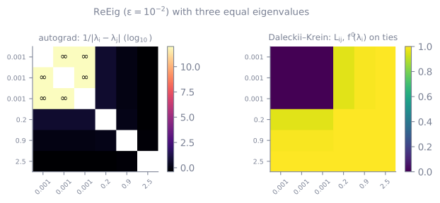
../_images/daleckii_krein.svg — After ReEig, three eigenvalues equal \(\epsilon\). Left: the factors \(1/|\lambda_i - \lambda_j|\) that autograd multiplies by are infinite on the tied block. Right: the Loewner matrix of the Daleckii–Krein backward is bounded (0 inside the clamped block, where \(f' = 0\)).¶

The two gradient paths. Each such operation exists as a snake_case function differentiated by autograd (logm_SPD, sqrtm_SPD, …) and as a CamelCase torch.autograd.Function with the backward above (LogmSPD, SqrtmSPD, …). Layers choose with use_autograd, False (manual) by default; the models accept a dict per layer type:

SPDnet(
    input_dim=8,
    hidden_layers_size=[4],
    output_dim=3,
    use_autograd={"bimap": True, "batchnorm": True},
)  # others stay manual

Valid keys: "bimap", "reeig", "logeig", "batchnorm", "vec", and "residual" for the residual models. The SPD linear algebra page lists the pairs.

Composite operations are built by chaining these primitives rather than by writing one large backward: the whitening, the means and the batch normalizations are compositions of manually differentiated steps, so each piece stays exact.

2. Matrix equations inside backward passes¶

Some backwards require solving a linear matrix equation. With \(A = V \operatorname{diag}(\alpha) V^\top \succ 0\), the Sylvester (Lyapunov) equation \(AZ + ZA = C\) has the closed form

\[ Z = V \left[ \frac{(V^\top C V)_{ij}}{\alpha_i + \alpha_j} \right]_{ij} V^\top \]

(solve_sylvester_SPD): the denominators are positive even when eigenvalues are equal. It appears in:

whitening \(X \mapsto G^{-1/2} X G^{-1/2}\) (the centring of the batch normalization): \(\bar X = G^{-1/2} \bar Y G^{-1/2}\), and the gradient with respect to \(G\) solves \(G^{1/2} Z + Z G^{1/2} = -2\,\mathrm{sym}\big(\sum_b \bar X_b X_b G^{-1/2}\big)\), summed over the batch (Whitening);
the Bures–Wasserstein exponential \(\mathrm{Exp}_B(V) = B + V + ZBZ\) with \(BZ + ZB = V\): differentiated implicitly (LyapunovSolveSPD), \(\bar V = W\) and \(\bar B = -(WZ + ZW)\) where \(BW + WB = \bar Z\);
the Bures–Wasserstein parallel transport from \(I\) to \(G\), the square root of the operator \(S \mapsto (GS + SG)/2\), whose derivative solves a Sylvester equation between operators with denominators \(b_{ij} + b_{kj}\), \(b_{ij} = \sqrt{(\delta_i + \delta_j)/2} > 0\) (ParallelTransportFromIdentityBW), finite even at \(G = I\).

3. Means as iterations¶

Mean	Computation	Notes
affine-invariant (Karcher)	\(M_{k+1} = M_k^{1/2} \exp\!\big(\eta_k \tfrac1N \sum_i \log(M_k^{-1/2} X_i M_k^{-1/2})\big) M_k^{1/2}\), \(\eta_k = 0.95^k\)	starts at \(I\); `mean_options={"n_iterations": 5}`
log-Euclidean	\(\exp\big(\tfrac1N\sum_i \log X_i\big)\)	closed form
arithmetic / harmonic	\(\tfrac1N\sum_i X_i\) / \(\big(\tfrac1N\sum_i X_i^{-1}\big)^{-1}\)	inverses through Cholesky
GAH	\(H \#_{1/2} A = H^{1/2}\big(H^{-1/2} A H^{-1/2}\big)^{1/2} H^{1/2}\)	closed form, close to the Karcher mean at the cost of two cheap means
adaptive GAH	\(H \#_t A\), \(t = \operatorname{sigmoid}(\tau)\) learned	\(t = 1/2\) at initialization
Bures–Wasserstein	\(G_{k+1} = G_k^{-1/2}\big(\tfrac1N\sum_i (G_k^{1/2} X_i G_k^{1/2})^{1/2}\big)^2 G_k^{-1/2}\)	from the arithmetic mean, one iteration by default

The iterations are unrolled, and the gradient flows through each of them with the manual spectral backwards. A small, fixed number of iterations is deliberate: the batch statistics only need to be good enough to normalize, and the backward cost grows with the number of iterations.

4. Implicit differentiation at a fixed point¶

An M-estimator of scatter is the fixed point \(\Sigma^\star = F(\Sigma^\star, x)\), with \(F(\Sigma, x) = \frac1n\sum_i u(x_i^\top \Sigma^{-1} x_i)\, x_i x_i^\top\). Differentiating the \(K\) unrolled iterations costs memory proportional to \(K\). At the fixed point, the implicit function theorem gives instead

\[ w = g + J_\Sigma^\top w, \qquad \bar x = J_x^\top w, \]

with \(g\) the upstream gradient and \(J_\Sigma\), \(J_x\) the Jacobians of \(F\). The library solves this adjoint equation by iteration, using only vector-Jacobian products (functions.m_estimators.MEstimator), so the memory cost does not depend on \(K\). Tyler’s estimator is scale invariant (\(F(c\Sigma) = cF(\Sigma)\), so \(J_\Sigma\) has the eigenvalue 1); normalizing the trace or the determinant at each iteration removes that direction.

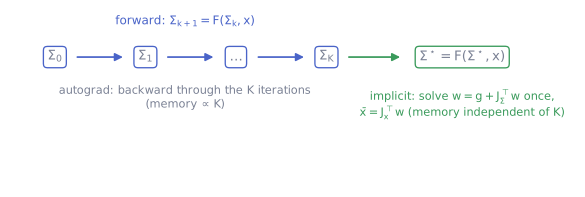
../_images/implicit_diff.svg — Unrolled vs implicit differentiation of a fixed point.¶

5. Parameters on manifolds without a Riemannian optimizer¶

Constraints are torch.nn.utils.parametrize parametrizations, so standard optimizers work unchanged (Layers and parametrizations has the equations of the static and dynamic modes):

orthonormal BiMap weights: orthogonal (static) or a QR / polar retraction of a tangent vector at a moving reference point (dynamic);
SPD biases: \(S \mapsto f(S)\) with \(f = \exp\) or the scaled softplus \(f(x) = \log_2(1 + 2^x)\), which satisfies \(f(0) = 1\): a zero parameter is the identity matrix;
positive scalars (the batch normalization scale \(s\)): scaled softplus; scalars in \((0, 1)\) (the adaptive GAH \(t\)): sigmoid.

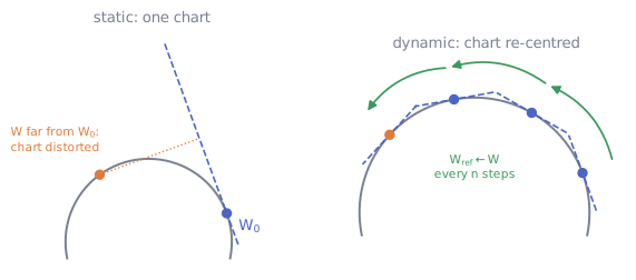
../_images/parametrization.svg — A static chart distorts the geometry far from its base point; the dynamic mode moves the base point to the current weight every `n_steps_ref_update` steps.¶

The reference point and the last value of an adaptive parametrization are separate buffers (clone()d): a buffer sharing the storage of the reference point would silently move it at every forward pass.

6. Batch normalization mechanics¶

Centring by whitening with the batch mean \(\bar X\) (a congruence, so affine-invariant distances within the batch are preserved), then re-biasing by the congruence with the learned \(G\) (Batch normalization).
Scaling (BatchNormSPDMeanScalarVariance): the centred matrices are raised to the power \(s/\sigma\), which moves them along the geodesics from \(I\) by the factor \(s/\sigma\); \(\sigma^2\) is the mean squared distance to the mean in the chosen geometry.
Running statistics follow the geometry: \(M_r \leftarrow M_r \#_\mu \bar X\) (geodesic step of size momentum \(\mu\)) and \(\sigma_r^2 \leftarrow (1-\mu)\sigma_r^2 + \mu\,\sigma^2\).
Minibatch smoothing (norm_strategy="minibatch"): normalize with \(m_k = m_{k-1} \#_{\mu_k} \bar X_k\) instead of \(\bar X_k\), to reduce the noise of small batches.
A batch of one matrix has no statistics (its mean is itself, its dispersion zero): it is normalized with the running statistics, which are not updated, and a warning is emitted.
GBWBN works in Bures–Wasserstein geometry, whose exponential at the identity \(\mathrm{Exp}_I(V) = (I + V/2)^2\) is only injective when \(I + V/2 \succ 0\). Outside that domain, a matrix is folded back and can come out numerically singular. The power \(\theta < 1\) compresses the spectrum and keeps most matrices inside the domain.

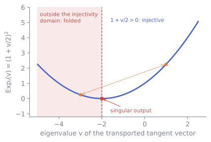
../_images/bw_fold.svg — The scalar picture of the Bures–Wasserstein exponential at the identity: beyond \(v = -2\) two tangent vectors give the same point, and \(v = -2\) gives a singular matrix.¶

7. The residual step¶

Unit step. The affine-invariant norm of the spectral vector field, \(\lVert V\rVert_X = \lVert X^{-1/2} V X^{-1/2} \rVert_F\), grows like \(1/\lambda_{\min}(X)\); an unnormalized step overflows on real covariances. The step is normalized to unit length, as in the reference implementation.
Cholesky instead of eigendecomposition for the norm: \(\lVert V \rVert_X = \lVert L^{-1} V L^{-\top} \rVert_F\) with \(X = LL^\top\) (two triangular solves).
Eigenvalue floor and projection. The block floors the eigenvalues of its input at \(10^{-8}\) (with the manually differentiated ReEig, the identity on well-conditioned inputs) and clamps those of its output to \([10^{-8}, 10^{8}]\) (projx).
Other geometries. A residual step can use any retraction \(X_+ = L\,\varphi(a\hat W)\,L^\top\) that agrees with \(\exp\) to first order: arithmetic \(1 + x\), harmonic \(1/(1-x)\), GAH \(e^{\operatorname{artanh} x}\) (see Riemannian residual networks).

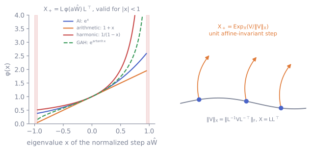
../_images/retractions.svg — Left: retractions of the residual step in whitened coordinates; all agree with \(e^x\) near 0 and are valid for \(|x| < 1\). Right: every matrix moves by one unit of affine-invariant distance.¶

8. ReEig and its variants¶

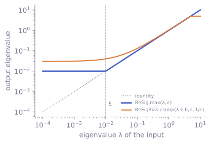
../_images/reeig.svg — ReEig clamps the eigenvalues below \(\epsilon\); ReEigBias shifts them by a learned \(b\) and clamps them to \([\epsilon, 1/\epsilon]\).¶

The derivative used in the Daleckii–Krein backward is \(f'(\lambda) = \mathbb{1}[\lambda > \epsilon]\): no gradient flows through the clamped directions, and the divided differences between a clamped and an unclamped eigenvalue interpolate between 0 and 1. \(\epsilon\) must match the scale of the data: eigenvalues below it are erased (for instance, HDM05 covariances are multiplied by 190 before an \(\epsilon = 0.8\) ReEig).

9. Precision and devices¶

float64 by default. The conditioning of real covariances reaches \(10^{6}\) (HDM05) to \(10^{7}\) (HyperLeaf); eigendecompositions and the divided differences lose too many digits in float32. Every function and layer takes dtype and device.
CPU vs GPU eigendecompositions. cuSOLVER’s eigh can fail to converge on nearly singular batches that LAPACK handles on CPU. For matrices of a few hundred rows, a CPU run with a few threads is often as fast as a small GPU.
Tests. The manual backwards are checked with torch.autograd.gradcheck in float64 and compared with the autograd path.