Layers and parametrizations

The SPDNet layers of yetanotherspdnet.nn, what they compute, and how their parameters are kept on their manifold. API: Layers, Parametrizations.

BiMap: the linear layer

BiMap maps a batch of SPD matrices to smaller SPD matrices by a congruence,

\[ X \in \mathcal{S}^{++}_{n_{in}} \;\longmapsto\; W^\top X W \in \mathcal{S}^{++}_{n_{out}}, \qquad W \in \mathbb{R}^{n_{in} \times n_{out}},\; n_{out} \le n_{in}. \]

The output stays SPD as long as \(W\) has full column rank. SPDNet constrains \(W\) to the Stiefel manifold \(\mathrm{St}(n_{in}, n_{out}) = \{W : W^\top W = I\}\), which rules out degenerate weights and keeps the scale of the data under control (parametrized=True, the default).

Static vs dynamic parametrization

A plain optimizer step \(W \leftarrow W - \eta \nabla_W \mathcal{L}\) leaves the Stiefel manifold. BiMap keeps \(W\) on it with a parametrization: the optimizer updates an unconstrained tensor \(\Xi\), and the layer uses \(W = \varphi(\Xi) \in \mathrm{St}\).

	parametrization_mode="static"	parametrization_mode="dynamic"
Trained tensor	\(\Xi \in \mathbb{R}^{n_{in}\times n_{out}}\)	\(\Xi \in T_{W_{ref}}\mathrm{St}\), a tangent vector
Weight	\(W = \varphi(\Xi)\), torch.nn.utils.parametrizations.orthogonal	\(W = \mathrm{qf}\big(W_{ref} + P_{W_{ref}}(\Xi)\big)\)
Reference point	none	\(W_{ref}\), moved every n_steps_ref_update steps
Needs	nothing	layer.register_optimizer_hook(optimizer)

Static. \(\varphi\) is fixed for the whole training. It is simple, but the parametrization distorts the geometry more and more as \(W\) moves away from where \(\varphi\) is well conditioned.

Dynamic. The trained tensor is a tangent vector at a reference point \(W_{ref}\). It is projected on the tangent space,

\[ P_{W}(\Xi) = \Xi - W\,\mathrm{sym}(W^\top \Xi), \qquad \mathrm{sym}(A) = \tfrac12 (A + A^\top), \]

then retracted on the manifold with the Q factor of a QR decomposition (or the polar factor, parametrization_options={"mapping": "polar"}). Every n_steps_ref_update optimizer steps, the reference point jumps to the current weight and the tangent vector is reset:

\[ W_{ref} \leftarrow W, \qquad \Xi \leftarrow 0 . \]

Each step is then a small move around the current point, where the retraction is accurate: a Riemannian optimizer implemented with a standard Euclidean one.

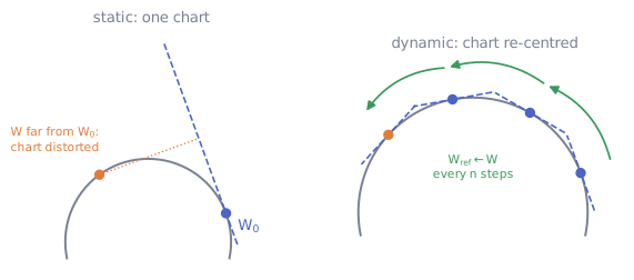
Static: one chart around the initial weight, increasingly distorted. Dynamic: the chart follows the weight.

Warning

Without register_optimizer_hook, the reference point never moves and the dynamic mode silently behaves like a static parametrization around the initial weight. The models forward the call to every dynamic layer: model.register_optimizer_hook(optimizer).

import torch
from yetanotherspdnet.nn import BiMap

layer = BiMap(n_in=64, n_out=32, parametrization_mode="dynamic", n_steps_ref_update=100)
optimizer = torch.optim.SGD(layer.parameters(), lr=1e-2)
layer.register_optimizer_hook(optimizer)  # moves W_ref every 100 steps

The same idea for SPD parameters

The bias of the batch normalization (and the GBWBN matrices \(M\), \(G\)) must stay SPD. SPDParametrization maps a symmetric \(S\) to \(f(S)\), with \(f\) applied to the eigenvalues: \(\exp\) ("exp") or the scaled softplus \(\lambda \mapsto \log_2(1 + 2^\lambda)\) ("softplus", the default, equal to 1 at 0). Its dynamic version, SPDAdaptiveParametrization, works around a reference point \(R\):

\[ B = R^{1/2}\, f\big(R^{-1/2} S R^{-1/2}\big)\, R^{1/2}, \]

with \(R \leftarrow B\) every n_steps_ref_update steps (batchnorm_parametrization_mode="dynamic" in the models).

ReEig and ReEigBias: the non-linearities

ReEig is the SPD analogue of ReLU: it clamps the small eigenvalues,

\[ X = U \operatorname{diag}(\lambda) U^\top \;\longmapsto\; U \operatorname{diag}\big(\max(\lambda_i, \epsilon)\big) U^\top . \]

Besides the non-linearity, it keeps the output conditioning bounded after a dimension reduction.

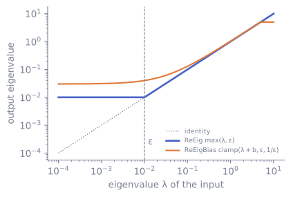
ReEig and ReEigBias as maps of the eigenvalues.

The threshold \(\epsilon\) (reeig_eps) must match the scale of the data: eigenvalues below it are erased.

ReEigBias adds a learned shift \(b_i\) per eigenvalue (in ascending order) and a two-sided clamp, \(U \operatorname{diag}\big(\operatorname{clamp}(\lambda_i + b_i, \epsilon, 1/\epsilon)\big) U^\top\); it starts as a two-sided ReEig (\(b = 0\)) and caps the condition number, which helps after estimators that can produce large eigenvalues.

LogEig, Vec, Vech: back to vectors

LogEig computes \(U \log(\Lambda) U^\top\). The logarithm maps the SPD manifold onto the vector space of symmetric matrices, where a Euclidean classifier makes sense. Vec flattens all \(n^2\) entries; Vech keeps the upper triangle, \(n(n+1)/2\) entries, which carry all the information of a symmetric matrix.

From samples to SPD matrices

SampleCovariance and MEstimation map raw samples (..., n_samples, p) to SPD matrices (..., p, p), differentiably with respect to the samples. The M-estimator down-weights outlying samples; see Covariance estimators for the estimators and their two gradient paths. They are the first layer of a network fed with raw signals or with CNN feature maps (covariance pooling).