Batch normalization

Euclidean batch normalization subtracts the batch mean, divides by the batch standard deviation, then applies a learned scale and shift. The SPD layers in yetanotherspdnet.nn.batchnorm do the same on the manifold, in the geometry chosen with mean_type (see Geometries on the SPD manifold).

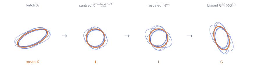
2×2 SPD matrices drawn as ellipses: the batch is centred (its mean becomes \(I\)), rescaled along geodesics from \(I\), then moved to the learned bias \(G\).

The two layers

BatchNormSPDMean

Centring and bias. Each matrix is transported so that the batch mean \(\bar X\) moves to the identity, then transported to a learned SPD bias \(G\) (Covbias). In the affine-invariant geometry this is \(X \mapsto G^{1/2}\,\bar X^{-1/2} X \bar X^{-1/2}\,G^{1/2}\). With mean_type="adaptive_geometric_arithmetic_harmonic", the batch mean is the point \(t\) of the affine-invariant geodesic from the harmonic to the arithmetic mean, with \(t = \operatorname{sigmoid}(\cdot)\) learned per layer (attribute t_gah, \(t = 1/2\) gives the GAH mean).

BatchNormSPDMeanScalarVariance

Centring, scalar dispersion and bias. Between centring and bias, the centred matrices are rescaled along geodesics from the identity by \(s / \sigma\): \(\sigma\) is the batch dispersion (a scalar, from <geometry>_std_scalar) and \(s\) a learned positive scalar (stdScalarbias). With mean_type="bures_wasserstein" this is GBWBN (Wang et al., 2025), which additionally learns a pre-transform \(X \mapsto M^{-1/2} X^\theta M^{-1/2}\) and its inverse, and learns its bias \(G\) on the input manifold, used as \(\hat G = M^{-1/2} G^\theta M^{-1/2}\) in the transformed space.

GBWBN options (bw_theta, bw_batch_stats_grad):

• bw_theta (default 0.5, the best value of the paper’s ablation): power deformation. The variance is that of the deformed metric, \(d_{BW}^2(X^\theta, Y^\theta) / \theta^2\). Since the BW metric is not scale invariant, \(\theta < 1\) also compresses the spectrum: with \(\theta = 1\) on ill-conditioned inputs, most transported tangent vectors \(V\) fall outside the injectivity domain \(I + V/2 \succ 0\) of \(\mathrm{Exp}_I\), and the centring is only approximate.

• bw_batch_stats_grad (default True, as in the paper): whether gradients flow through the batch mean and variance. False treats them as constants, as the reference implementation does.

In the models, pass them as batchnorm_bw_options={"bw_theta": 0.25}.

Note

The GBWBN parameters \(M\) and \(G\) start at the identity, where all eigenvalues are equal. Gradients through torch.linalg.eigh are undefined there, so keep use_autograd=False (the default) for this layer: the manual backwards (Daleckii–Krein for \(M^{\pm 1/2}\) and \(M^\theta\), implicit differentiation for the Lyapunov solve and the transport to \(\hat G\)) stay finite and exact at the identity.

In the models (SPDnet, RResNet, GBWBNRResNet) these correspond to batchnorm_type="mean_only" and batchnorm_type="mean_var_scalar", and every layer option is exposed with a batchnorm_ prefix.

Training and evaluation

Mode	Statistics used	Running statistics
model.train(), batch of ≥ 2 matrices	batch mean (and dispersion)	updated with momentum
model.train(), a single matrix	running mean (and dispersion)	not updated, a UserWarning is emitted
model.eval()	running mean (and dispersion)	not updated

A batch of one matrix has no batch statistics: its mean is the matrix itself and its dispersion is zero, so normalizing with them would map every input to the identity. Such batches (for instance a last incomplete batch of size 1) are therefore normalized like in evaluation mode. Use drop_last=True in your DataLoader to avoid them entirely.

Main options

momentum

Update rate of the running statistics: running = geodesic(running, batch, momentum).

norm_strategy

"classical" normalizes each batch with its own mean. "minibatch" normalizes with a smoothed mean m_k = geodesic(m_{k-1}, batch_mean, minibatch_momentum_k), where \(m_{k-1}\) is the mean used for the previous batch. This reduces the noise of small batches. The step minibatch_momentum_k follows minibatch_mode ("constant", "decay" towards minibatch_momentum, or "growth" from it) over minibatch_maxstep steps.

parametrization, parametrization_mode

How the SPD bias stays SPD: "softplus" or "exp" maps on the eigenvalues. The "dynamic" mode re-centres the parametrization on the current value every n_steps_ref_update optimizer steps. It requires layer.register_optimizer_hook(optimizer) after creating the optimizer.

mean_options

Extra arguments of the mean function, for instance {"n_iterations": 5} for the affine-invariant and Bures–Wasserstein means.